Multiple Linear Regression Walkthrough

📥 Data Import & Description

import pandas as pd
import numpy as np
import seaborn as sns
import matplotlib.pyplot as plt

dataset = pd.read_csv('Student_Performance.csv')

We work with a dataset of 10,000 students, containing:

• 4 continuous variables
• 1 binary categorical variable (Extracurricular Activities)
• 1 target variable (Performance Index)

🔍 Exploratory Data Analysis (EDA)

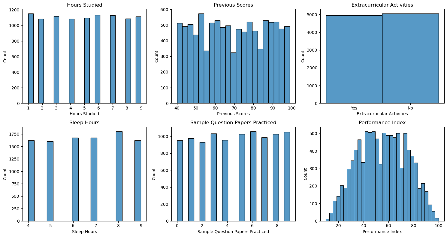
We start by analyzing data types, distribution, and visualizing feature relationships with the target variable.

Distributions

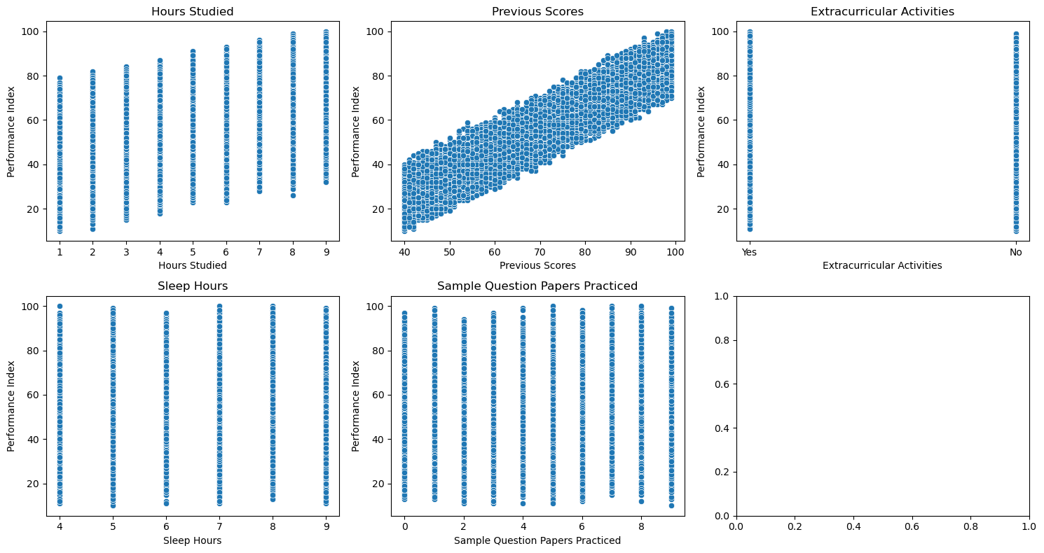
Scatter Plots vs Target

Correlation Heatmap

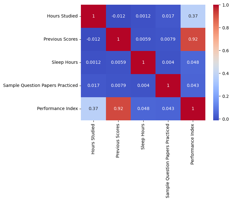
Insights:

• Previous Scores have a very strong positive correlation (0.92) with Performance Index.
• Hours Studied has a moderate positive correlation (0.37).
• No multicollinearity issues among features.

🧹 Data Preprocessing

Binary Encoding for Extracurricular Activities:

dataset['Extracurricular Activities'] = dataset['Extracurricular Activities'].map({'Yes': 1, 'No': 0})

Standardization for continuous variables:

from sklearn.preprocessing import StandardScaler

scaler = StandardScaler()
cols = ['Hours Studied', 'Previous Scores', 'Sleep Hours', 'Sample Question Papers Practiced']
dataset[cols] = scaler.fit_transform(dataset[cols])

✂️ Train-Test Split

from sklearn.model_selection import train_test_split

X = dataset.drop("Performance Index", axis=1)
y = dataset["Performance Index"]

X_train, X_test, y_train, y_test = train_test_split(X, y, test_size=0.2, random_state=13)

🧠 Model Fitting

from sklearn.linear_model import LinearRegression

model = LinearRegression()
model.fit(X_train, y_train)

Model Coefficients

print(pd.Series(model.coef_, index=X.columns))

Equation of the fitted model:

Y = β₀ + β₁·X₁ + β₂·X₂ + β₃·X₃ + β₄·X₄ + β₅·X₅

• X₁ = Hours Studied
• X₂ = Previous Scores
• X₃ = Extracurricular Activities
• X₄ = Sleep Hours
• X₅ = Sample Question Papers Practiced

📊 Model Evaluation

from sklearn.metrics import mean_absolute_error, mean_squared_error, r2_score

mae = mean_absolute_error(y_test, y_pred)
mse = mean_squared_error(y_test, y_pred)
rmse = np.sqrt(mse)
r2 = r2_score(y_test, y_pred)

Results:

• MAE: 1.622
• MSE: 4.144
• RMSE: 2.036
• R² Score: 0.989

📈 Residual Analysis

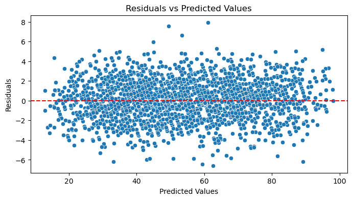
Residuals are evenly spread around 0 ; no pattern detected. Indicates assumptions of linearity and homoscedasticity hold.

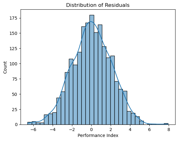
Residuals appear normally distributed ; supports the assumption of normality.